Mathematics with Maple

S.Duzhin

Lesson 4: Derivative and Taylor series

Mathematics: derivative of a function, Taylor expansion.

Maple: diff, animate.

In English, the noun "derivative" is related to the verb "to differentiate": to differentiate a function means to find its derivative.

This verb gives the name to the Maple command that finds the derivative of a function: diff.

Let us try it on some simple examples:

> diff(x^2,x);

> diff(sin(x),x);

Exercise 1.

Find the derivative of the function y=x^x and its value at the point x=1.

The second argument of the command diff is the name of the variable with respect to which you differentiate. If the function depends on several variables, like f(x,y), you can find the derivative with respect to any one of them:

> diff(x^2+x*y+y^2,x);

> diff(x^2+x*y+y^2,y);

Exercise 2.

Find a function z=f(x,y) such that dz/dx=2*x*y, dz/dy = x^2+1

Exercise 3.

Is there a function z=f(x,y) that satisfies dz/dx=x*y, dz/dy=x*y?

The physical meaning of the derivative f'(x) is the speed with which the values of the function f(x) change when x changes. The geometrical meaning of the derivative is the slope of the graph of the function.

The behaviour of the derivative is determined by the behaviour of the function so that

if the function y(x) is constant (-) then the derivative is 0;

if the function y(x) is increasing (/) then the derivative is >0;

if the function y(x) is decreasing (\) then the derivative is <0.

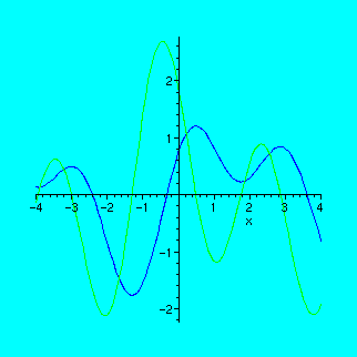
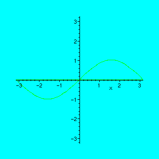
Look carefully at the following graph of the function and its derivative and make sure that these rules are satisfied:

> f:=sin(x)+1/2*sin(2*x+1)-1/3*sin(7/3*x-2);

> fd:=diff(f,x);

> plot({f,fd},x=-4..4);

Exercise 4.

Look at the following graph:

> plot(cos(x)-2*sin(2*x-1),x=-3..3);

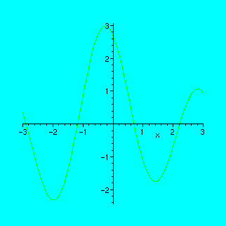
Print this graph on a printer, then draw the graph of the derivative on the same sheet of paper BY HAND, then check your result by plotting the graph of the derivative with Maple.

Now let us recall the rigorous definition of the derivative and try to vizualise it with Maple.

The derivative of the function y=f(x) is a new function y=f'(x) such that its value at any point x0 is equal to the limit of (f(x)-f(x0)/(x-x0) as x --> x0:

> f:='f';

> Limit((f(xm)-f(x0))/(xm-x0),xm=x0);

The notation xm suggests a "moving" point: the point xm moves along the x-axis towards the fixed point x0.

Denote y0=f(x0). The point (x0,y0) lies on the graph of the function f.

If you draw the line in the (x,y)-plane through the point (x0,y0) with the angle coefficient (f(xm)-f(x0))/(xm-x0), you will obtain the secant -- a straight line that passes through (x0,y0) and one more point of the graph, (xm,f(xm)). Whe xm moves towards x0, the secant tends to the tangent. The value of y'(x0) is the angle coefficient of the tangent line.

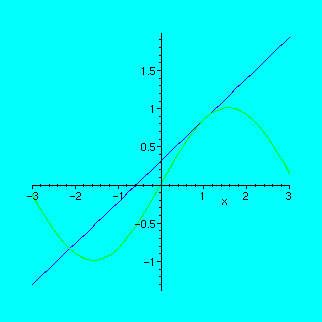
Let us draw a function and the tangent line to its graph on one plot:

> x0:=1;

> plot({sin(x),sin(x0)+cos(x0)*(x-x0)},x=-3..3);

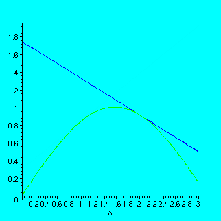
We can also draw several tangents on the same picture:

> x1:=2;

> plot({sin(x),sin(x0)+cos(x0)*(x-x0),sin(x1)+cos(x1)*(x-x1)},x=0..3);

Exercise 5.

Plot the graph of the function from Exercise 4 and its tangents at points x0=0 and x1=1.

Now let us watch the motion of secants towards the tangent

using the Maple procedure "animate". Before using it, we have to load the corresponding package:

> with(plots);

This command gives you the list of all names available in this package, among them you see "animate".

We will see how the secant to the graph of sin(x) moves towards the tangent at point x0=1:

> x0:=1;

> animate({sin(x),k*x},x=-Pi..Pi,k=0..1,frames=40);

Try to experiment with the buttons of the animation window! It is like an ordinary tape-recorder: you can change the direction, rewind, stop, restart etc.

OK. Now let us look at this procedure from another viewpoint.

Let y=f(x) be a curve in the plane (x,y) and (x0,y0), where y0=f(x0), a point on this curve.

Consider all the straight lines passing through the point (x0,y0)=P.

The general equation of such lines is

y=y0+a*(x-x0) (1)

where a is the angle coefficient.

Which of these straight lines is most close to the given curve

near the point P?

Answer: it is the tangent given by the equation y=y0+f'(x0)*(x-x0)

(take a=f'(x0) in the general equation (1)).

Now let us consider a bigger family of simple lines: all quadratic curves that pass through the fixed point P and try to understand which one of them is most close to our curve y=f(x).

A quadratic curve is determined by this equation:

y = y0+a*(x-x0)+b*(x-x0)^2

so there are two parameters: a and b which we can change.

In any Maple animation, there is only one parameter, so let us do several animations and try to understand the meaning of the two coefficients.

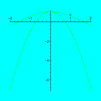
In the example below, I take the function y=cos(x) at the point x0=0, y0=1.

First, we fix b=1 and change a from -1 to 1:

> b:=1;

> animate({cos(x),1+a*x+b*x^2},x=-2..2,a=-1..1);

You see that the parabola becomes especially close to the cosine line when a=0.

Now let us fix a=0 and move the value of b from 0 to -2.

> a:=0;

> b:='b';

> animate({cos(x),1+a*x+b*x^2},x=-2..2,b=-2..0);

You have noticed that for one specific value of a, the parabola gets especially close to our curve. What is this value?

If you work with the "tape-recorder" in "discrete" mode (pressing the "frame-advance" button to the right of the usual "play" button), you can count the number of times you press the button. Since there are 16 frames all in all, and the best approximation is achieved at the forth stroke, the corresponding value is a=-1/2.

Thus, we have found the following experimental result:

among all parabolas y=1+a*x+b*x^2, the parabola

y=1-1/2*x^2 is most close to the curve y=cos(x).

Exercise 6.

Find the values of a and b in the equation of the parabola y=-1+a*x+b*x^2 which is most close to the graph of the function y=-(1-x^2)^(1/2) near the point x0=0.

The polynomial 1-1/2*x^2 is the Taylor series for the function y=cos(x) truncated at degree 2.

Let me remind you the general definition of the Taylor series.

The Taylor series of the function y=f(x) at the point x0 is the following infinite series:

t = f(x0) + f'(x0)*(x-x0) + f''(x0)/2*(x-x0)^2 + f'''(x0)/6*(x-x0)^3 + ...

where the numbers in denominator are 1!=1, 2!=2, 3!=6, ...

The meaning of the Taylor series is that it gives the best polynomial approximation to the given function near the point x0.

The Maple command to find Taylor expansion is taylor. It normally takes three arguments: the function, name of the variable and the order.

Here is an example:

> taylor(cos(x),x,8);

You see that the beginning of the series (1-1/2*x^2) is the parabola that we found in our experiments!

Now let us draw the graphs of some truncated Taylor series for the function cos(x) and see that they are VERY close to the graph of the function NEAR the chosen point.

> p0:=1; # order 0

> p2:=p0-1/2*x^2; # order 2

> p4:=p2+1/24*x^4; # order 4

> p6:=p4-1/720*x^6; # order 6

> plot([cos(x),p2,p4,p6],x=-4..4,color=[yellow,red,green,blue]);

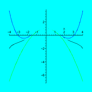
On this picture, the graph of cos(x) is yellow, p2 is red, p4 is green and p6 is blue. You can see that p2 is close to cosine, p4 more close, and p6 is the most close NEAR the point x0=0.

To see how close the graphs of p2, p4 and p6 are to the graph of cos(x), it is useful to plot the differences:

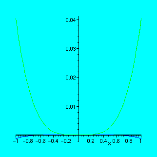
> plot([cos(x)-p2,cos(x)-p4,cos(x)-p6],x=-1..1,color=[red,green,blue]);

Exercise 7.

Find the Taylor expansion to order 7 of the function y=-(1-x^2)^(1/2)

near point x0=0 and plot the graphs of the function itself and the Taylor approximations of order 2, 4 and 6. Submit a printout to the teacher.

Exercise 8.

Find a function z=f(x,y) such that dz/dx = -y/(x^2+y^2), dz/dy = x/(x^2+y^2).

Exercise 9.

Find the Taylor series expansion of the function y=exp(-1/x^2).

Plot the graph of the function itself and some Taylor polynomials.

Can you explain what you see?

Exercise 10.

We have not yet studied Maple programming, but...

Below is the Maple procedure to see animated Taylor expansions.

Try to understand how to use it (do not forget to convert it to Maple input first).

taylorpic := proc(func,xrange,n)

local picture,x,y,a,b,i,p,q,taylorfunc,delay,j,v;

if nargs = 4 then delay := args[4]; v := NULL;

elif nargs = 5 then delay := args[4]; v:= args[5];

else delay := 1; v := NULL;

fi;

x := op(1,xrange);

y := op(2,xrange);

a := op(1,y); b := op(2,y);

delay := [seq(delay,j=1..n)];

for i from 1 to n do

taylorfunc:= convert(taylor(func,x,i),polynom);

p := plot({func,taylorfunc},x=a..b,color=green);

q := plots[textplot]([(a+b)/2,6.5,`Taylor Expansion to order = `.i], color=red);

p := plots[display]({p,q});

picture[i] := seq(p,j=1..delay[i]);

od;

plots[display]([seq(picture[i],i=1..n)],insequence=true,v);

end: