![[Maple Math]](images/lesson092.gif)
Mathematics with Maple
S.Duzhin
Lesson 9: Conics and Quadrics
Mathematics: conic, quadric, normal form.
Maple: plot3d, implicitplot, display.
List of key words:
conic (curve of second order),
quadric (surface of second order),
ellipse,
hyperbola,
parabola,
ellipsoid,
hyperboloid of one sheet,
hyperboloid of two sheets,
elliptic paraboloid,
hyperbolic paraboloid,
conic surface,
cylinder.
To any equation in two variables f(x,y)=0, you can assign the set of all points in the plane whose coordinates (x,y) satisfy this equation. This procedure can be visualized in Maple using the command implicitplot from the package plots.
Here is an example:
> with(plots):
> f1:=(x^2+y^2-25)*(abs(x-2)+abs(x+2)-4+(y+3)^2)*(x^2+abs(y-1)+abs(y+2)-3)*((x+3)^2+1/2*(y-3/2)^2-1)*((x-3)^2+(y-2)^2-1);
![]()
![[Maple Math]](images/lesson092.gif)
> implicitplot(f1=0,x=-5..5,y=-5..5,axes=none,numpoints=3600);

The additional parameters "axes=none" and "numpoints=3600" are optional; you can try to repeat the command without them. Increasing the value of numpoints leads to a better resolution.
Similarly, any equation f(x,y,z) = 0 with three unknowns determines a set of points in the 3-dimensional space. The corresponding Maple command is implicitplot3d. An example:
> implicitplot3d(x^2+y^2/4+(z-1)^2=1,x=-2..2,y=-3..3,z=-1..3,style=patchnogrid);
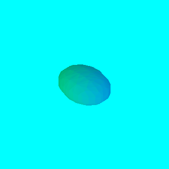
In general, if the function f(x,y) is "good", then the corresponding point set in the plane is a _curve_. Similarly, if f(x,y,z) is "good", then we obtain a _surface_ in the space.
Let us explore the SIMPLEST possible equations in 2 and 3 variables and thus see what are the simplest curves and surfaces that exist.
You may agree that simplest expressions are those that contain only addition and multiplication, i.e. polynomials. Polynomials do not contain such "bad" expressions as sin, exp, log, sqrt and even 1/x.
Polynomials themselves can be arranged by their degree. Let me write down the general form of a polynomial in two variables of degree 1, 2 and 3:
> p1 := a1*x + a2*y + a0;
![]()
> p2 := a11*x^2 + a12*x*y + a22*y^2 + a1*x + a2*y + a0;
![]()
> p3 := a111*x^3 + a112*x^2*y + a122*x*y^2 + a222*y^3 + a11*x^2 + a12*x*y + a22*y^2 + a1*x + a2*y + a0;
![]()
Here a0, a1, a2, a11, ... are some real numbers (constants).
If you substitute specific values of these constants, you will get a concrete equation and hence a concrete curve which can be displayed with implicitplot.
In degree 1 everything is very simple:
any curve of first order is a straight line, e.g.:
> f:=subs({a1=3,a2=-2,a0=1},p1);
![]()
> implicitplot(f,x=-2..2,y=-2..2);
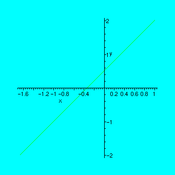
Choosing different values for a0, a1 and a2 will give a straight line with another position in the plane, but it will be a straight line still.
In degree 2 the situation is much more interesting: choosing different values of the parameters, you can get completely different pictures.
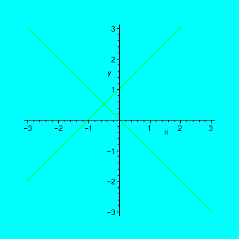
Two lines:
> f := y^2-x^2-y-x;
![]()
> implicitplot(f=0,x=-3..3,y=-3..3,numpoints=2500);
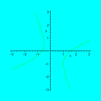
A hyperbola:
> implicitplot(x^2-2*x*y-y^2-x=1,x=-3..3,y=-3..3);
An ellipse:
> implicitplot(x^2+2*x*y+3*y^2-x=1,x=-3..3,y=-3..3);
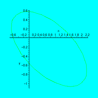
From the course of linear algebra you may remember that any curve defined by a second order equation
a11*x^2 + a12*x*y + a22*y^2 + a1*x + a2*y + a0 = 0
can belong to one of the following 8 types:
ellipse, hyperbola, parabola, two intersecting lines, two parallel lines, one line, one point, empty set.
Curves in the plane that can be defined by a second order equation are also called CONICS, or CONIC SECTIONS. Usually this name is used only for the first 3 types in the list: ellipse, hyperbola, parabola -- which are called non-degenerate conics (because, if you remember, the matrix of the corresponding quadratic form has nonzero determinant in this case).
Exercise 1.
Determine the type of the curves below by drawing its picture with implicitplot
A. 3*x^2-4*x+2*x*y-y^2 = 0.
B. x^2+x+4*x*y+2*y+4*y^2 = 0.
C. 2*x^2-2*x*y+5*y^2+2*x+1-4*y = 0.
D. x^2+2*x*y+y^2+1-2*y = 0.
Now let us do some animated cartoons which will help us to understand how the gradual change of parameters affects the form of the conic. With the implicit plots, you cannot use the command "animate", and the correct way to do it is first to prepare the necessary graphical data as a sequence of images, and then to display it.
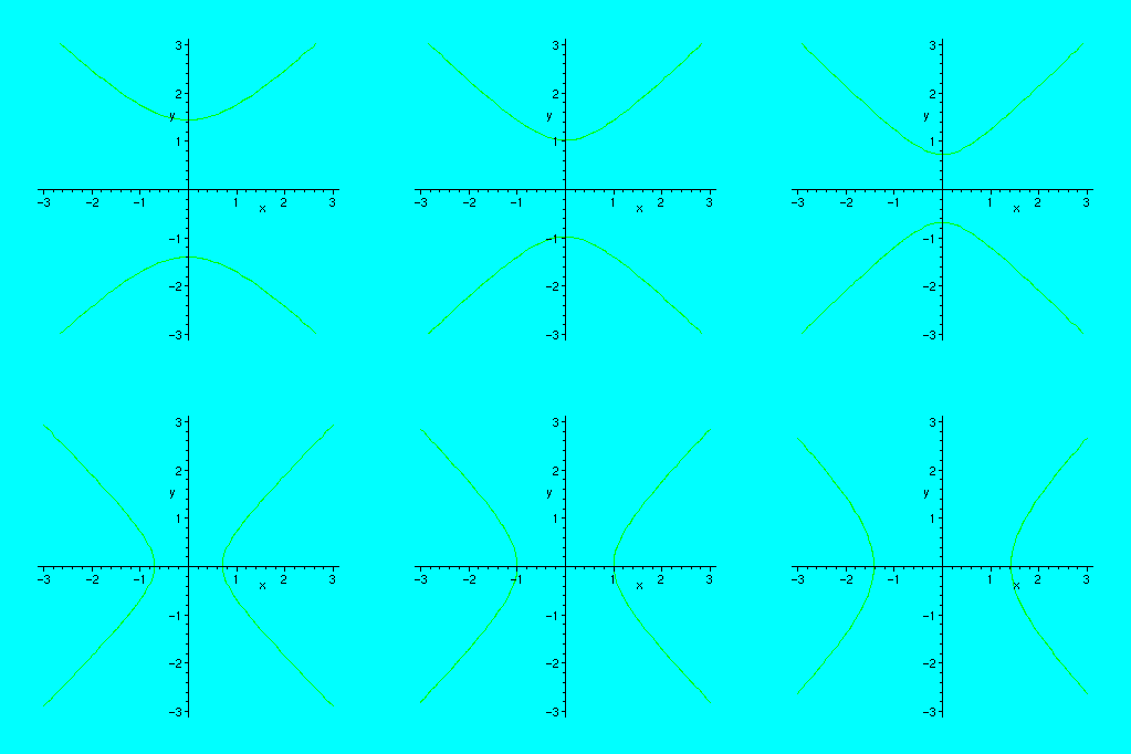
Example. Animating the curve x^2 - y^2 = c , when c varies from -2 to 2 by steps of 0.5.
Since the parameter in seq must be integer, we write x^2-y^2=a/2 and take integer values for a, then c will take values -2.0, -1.5, -1.0, ... ,2.0
> P:=seq(implicitplot(x^2-y^2=a/2,x=-3..3,y=-3..3),a=-4..4):
The previous command takes some time, but then the next one is quite fast:
> display([P],insequence=true);
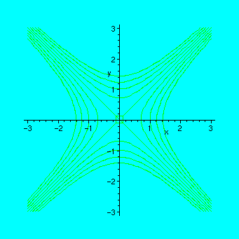
You can also try it without the option "insequence=true", but the result will not be so exciting:
> display([P]);
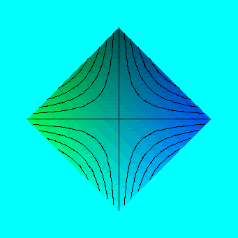
Another way to see how the shape of the curve changes is to draw a 3-dimensional graph with option
> plot3d(x^2-y^2,x=-3..3,y=-3..3,orientation=[45,0],style=patchcontour);
Exercise 2.
A. Following the example above, make up the command to watch the evolution of the curve 2*x^2+2*x*y+2*x+y^2+2*y+1 = a, when "a" changes from 0 to 4.
B. Find an equation of second order with parameter "a" which gives an ellipse when a>0, a parabola when a=0 and a hyperbola when a<0.
Now let us have a look at QUADRICS (surfaces of second order in 3-dimensional space). They are given by an equztion of the form f(x,y,z)=0 where f(x,y,z) is a polynomial of degree 2 in 3 variables.
The general form of such polynomial is:
> q:=a11*x^2 + a22*y^2 + a33*z^2 + a12*x*y + a13*x*z + a23*y*z + a1*x + a2*y + a3*z + a0;
![]()
The number of different possibilities in this case is bigger than in the plane. The classification theorem for quadrics in 3-space says:
Any surface given by the equation q=0 belongs to one of the following 14 types:
ellipsoid, hyperboloid of one sheet, hyperboloid of two sheets, elliptic paraboloid, hyperbolic paraboloid, conic surface, elliptic cylinder, hyperbolic cylinder, parabolic cylinder, 2 intersecting planes, 2 parallel planes, 1 plane, 1 point and empty place.
The first 9 types are called non-degenerate, and they represent genuine curvilinear surfaces; the last 5 types are made up of straight-line objects.
The theorem of linear algebra also says that by an appropriate linear change of variables, you can rewrite the equation of every surface in normal (or canonical) form. Let me give the normal forms of the first six (most interesting) types of surfaces so that you can see all of them on your screen:
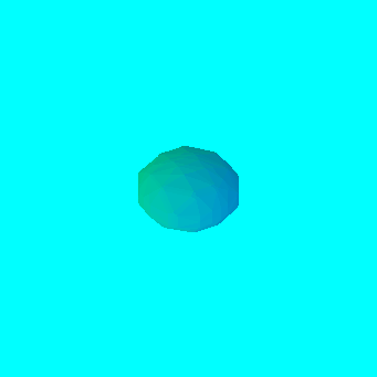
1. ellipsoid (its canonical form is just a sphere):
> f:=x^2+y^2+z^2-1;
![]()
> implicitplot3d(f,x=-2..2,y=-2..2,z=-2..2,style=patchnogrid);
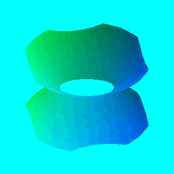
2. hyperboloid of one sheet:
> f:=x^2+y^2-z^2-1;
![]()
> implicitplot3d(f,x=-2..2,y=-2..2,z=-2..2,style=patchnogrid);
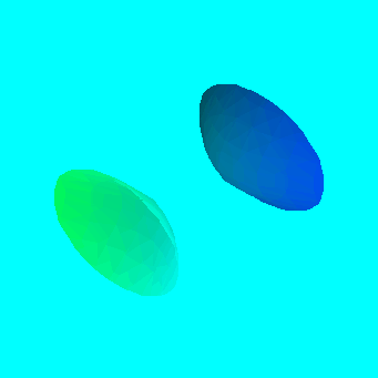
3. hyperboloid of two sheets:
> f:=x^2-y^2-z^2-1;
![]()
> implicitplot3d(f,x=-2..2,y=-2..2,z=-2..2,style=patchnogrid);
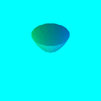
4. elliptic paraboloid:
> f:=x^2+y^2-z;
![]()
> implicitplot3d(f,x=-2..2,y=-2..2,z=-2..2,style=patchnogrid);
5. hyperbolic paraboloid:
> f:=x^2-y^2-z;
![]()
> implicitplot3d(f,x=-2..2,y=-2..2,z=-2..2,style=patchnogrid);
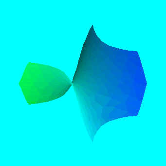
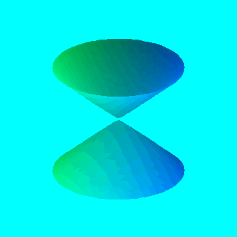
6. conic surface:
> f:=x^2+y^2-z^2;
![]()
> implicitplot3d(f,x=-2..2,y=-2..2,z=-2..2,style=patchnogrid,numpoints=3600);
>
Remarks 1. In cases 4 and 5, a better quality of the plot can be achieved by using plot3d instead of implicitplot3d.
Remark 2. The conic surface (6) has a SINGULAR point at (0,0,0). Near this point, the picture is not very good. To make it more correct, try to increase the resolution by adding "grid=[20,20,20]" (also try bigger values).
Exercise 3.
Using Maple, determine the type of each of the following surfaces:
a. 7x^2+6y^2+5z^2-4xy-4yz-6x-24y+18z+30=0;
b. 2x^2+2y^2-5z^2+2xy-2x-4y-4z+2=0;
c. x^2+5y^2+z^2+2xy+2yz+6zx-2x+6y+2z=0.